👨🏫 Notes on Lecture 10
Formulas for this lecture can be found in my paper formula sheets and online formula sheet.
Formulas for this lecture can be found in the formula sheet.
Optimal Diversification
As you add more stocks to your portfolio, the risk in your portfolio, measured as standard deviation (σ), decreases:
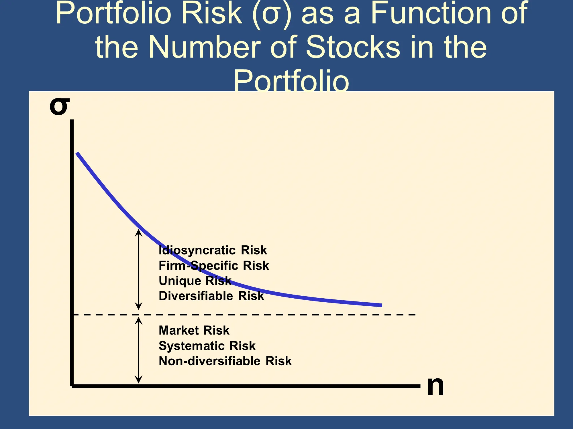 |  |
However, it doesn’t decrease down to zero. Rather, it approaches a floor level of “market risk.”
This allows us to divide all of the risk in our portfolio into two types:
- Idiosyncratic/Firm-Specific/Diversifiable Risk - with proper diversification, we can remove this risk from our portfolio. The more stocks we add to our portfolio, the more of the idiosyncratic risk we can remove.
- Market/Systematic/Non-diversifiable Risk - this type of risk can’t be “diversified away” by adding more stocks and bonds. Note for later: β is a measure of the market/systematic/non-diversifiable risk of a stock (or of a portfolio of stocks).
It’s pretty amazing that diversification (which is free) can significantly reduce the idiosyncratic risk in your portfolio. How does it do that? Diversification works because if one of your securities “does poorly,” there is a good chance that another security “does well,” and this can lessen the total risk in your portfolio. The good performance of the second security can “dull the pain” from the first security. This is, fundamentally, all that diversification is about.
This explanation assumes that when the first security does poorly, the second security tends to do well, to counterbalance the first. If this is the case, the securities are said to be “negatively correlated,” because the two securities have opposite performances (ie when one has a lower return than it usually has, the other has a higher return than it usually has). Negatively correlated securities provide less diversification, because losses by one security tend to be cancelled out by gains in other securities.
As we’ve seen, negative correlation is good for investors because it allows one security to provide a form of insurance against risk in another security. Unfortunately, negative correlation is fairly rare. In fact, typically, the IRR/return on assets with negative correlation with the market is negative. In other words, rather than earning money when you invest in them, they typically cost you money on average. Just as you must pay for health insurance or car insurance, you must pay for negative correlation.
What is far more common is positive correlation. Diversification still works with positive correlation, but it is not as effective. Security A and Security B are positively correlated if, when Security A does below average, Security B is more likely to also do below average. To see why this leads to poor diversification, imagine you had a considerable amount of money invested in Security A. You are worried about the risk of security A losing money (having a negative return). Therefore, you transfer some of your money from Security A to Security B. This will provide a tiny bit of diversification because if Security A has a low return, Security B might have a high return. However, because they are positively correlated, it is more likely that Security B will also have a low return. For example, suppose you are concerned about a loss of 10% on Security A. If you attempt to diversify to Security B and security B also has a loss of 10%, then your portfolio will still have a loss of 10%. You will have had no benefits of diversification.
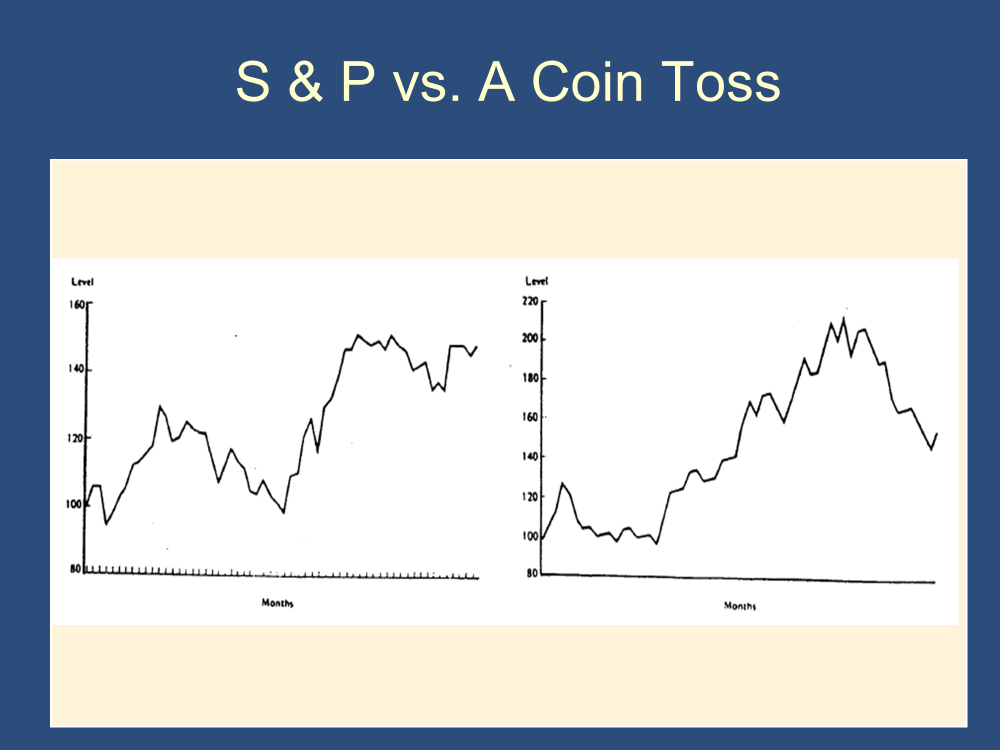
This is what Bruce means in the following slide:

The limits to diversification come from the fact that various securities are typically correlated. Much of the performance of any given stock on any given day can be predicted by how the Dow Jones Average does on that day. If the Dow is down, the vast majority of stocks will also be down. Therefore, diversifying into many, many stocks won’t save you from a day on which the Dow is down. This, fundamentally is what systematic risk is. It’s based on the fact that all securities tend to move together, so they can’t cancel losses out from the other securities as well as we might hope.
The concept of correlation is precisely defined in probability, statistics, data science, advanced finance, and many other courses. It can be calculated from historical data, but you are not responsible for knowing how in this class. However, for reference, here are the correlations between some common stocks and a portfolio with all US stocks:
| Correlation with the VTI ETF | |
| Amazon | 59% |
| IBM | 58% |
| Disney | 74% |
| Microsoft | 62% |
| Boeing | 58% |
| Starbucks | 58% |
| ExxonMobil | 59% |
When stocks are negatively correlated, the number for mathematical correlation is negative. As you can see the stocks above are quite significantly correlated with the US stock market as a whole.
Ray Dalio breaks down his “Holy Grail”
The Capital Asset Pricing Model (CAPM)
The CAPM is a mathematical model that says that under certain assumptions, the expected returns that investors demand for a stock are determined by the systemic risk (β) that the stocks have.
The CAPM is a mathematical theory that says that there is a tradeoff between risk and higher returns. This is captured in the following formula, where β represents risk and represents the return on a specific Stock. Note that the return in the
There is a formula for beta that can be used to estimate beta using historical data. Intuitively, however, Beta represents a “non-diversifiable risk.”
Investors don’t want to be exposed to risk, and they especially don’t want to be exposed to non-diversifiable risk Within the assumptions of the CAPM, investors can and will diversify away the idiosyncratic risk. Therefore, investors don’t care about idiosyncratic risk - they only care about systematic risk, which is captured in β. This is why β completely determines expected returns in the CAPM.
Side note:
To understand the CAPM, you need to understand that the CAPM is a mathematical model much like the money multiplier model is a model. Like the money multiplier model, the CAPM is a useful model that can help us understand why things happen the way that they happen.
Like the money multiplier model, the CAPM is based on certain assumptions. Those assumptions are that everyone starts with roughly the same beliefs about the world and that these beliefs are largely true. Likewise, the CAPM assumes that everyone is very sophisticated about diversification and that there are many securities to invest in. It uses the tools of supply and demand and probability theory to investigate what drives securities prices.
What does this mean for you? Just know that there is a lot of modeling that has been done, and when similar assumptions are used, similar conclusions are arrived at. We want to get a sense of those assumptions and those conclusions. That’s all we need to do!
Fundamentally, the above equation tells you the expected rate of return that investors will require if they are going to be willing to invest in/hold the security.
Values of Beta:
- For the market as a whole,
- implies stock requires a return greater than the market return, because the stock is riskier (has a higher standard deviation) than the market
- implies stock requires a return lower than the market return, because the stock is less risky (has a lower standard deviation) than the market
The main skill you’ll need to develop is applying the main CAPM formula.
| Stock | Beta | |
| Amazon | 2.20 | 20.4% |
| IBM | 1.59 | 16.1% |
| Disney | 1.26 | 13.8% |
| Microsoft | 1.13 | 12.9% |
| Boeing | 1.09 | 12.6% |
| Starbucks | .69 | 9.8% |
| ExxonMobil | .65 | 9.6% |
Assume that
- the risk-free rate
- the expected return on the market portfolio Therefore, the expected risk premium on the market
The above table says that Amazon has a huge amount of non-diversifiable risk . Therefore, within the CAPM model, investors won’t be willing to own it unless they have an expected return of 20.4% when owning Amazon:
✏️ Suppose that that Meta has β=1.3. What is the expected return on Meta, based on the above assumptions.
✔ Click here to view answer
⚠️ This is a potential ‘gotcha’ on the exam.
✏️ Suppose that the risk premium on the market was 9% instead of 7%. What would the expected return on Meta be?
✔ Click here to view answer
Here, we are given , so we just plug it directly into the formula:
Whenever you see the phrase, “risk premium” make sure to look the term up in the following Jargon cheat sheet.
Jargon cheat sheet
✏️ You are evaluating a risky stock. You expect the stock to have a return of 17%, but because the stock is so risky, you don’t know if it is actually a good investment. You expect the overall market to have a return of 12%. The risk free rate is 2% and the beta for this stock is 2.4. What return would the CAPM expect for this stock? Is it a good investment?
✔ Click here to view answer
, ,
The CAPM predicts that this stock is risky enough that it should have a return of 26%.
However, your analysis suggests that it will only have a return of 17%. That’s not enough to compensate you for the riskiness of the stock. Therefore, it’s a bad investment.
Applications of the CAPM
- Calculating required rates of return to calculate discount rates.
- Performance evaluation of portfolio managers (calculate the return they should be earning based on the beta of their portfolio and then compare their actual results to that prediction.)
- A way to conceptualize investment decisions and to understand diversification.
Fundamental analysis: Attempt to determine a stock’s fundamental value by analyzing the company, the industry, and the macroeconomy. Technical analysis: looking at stock price charts to find and exploit recurring and predictable patterns
Efficient Market Hypothesis
EMH:
- Markets incorporate all available information immediately into a security’s price.
- This means that the security’s price represents the market’s best guess of the security’s future price, taking into account any income earned along the way.
- Securities are never mispriced, so there earn above-average returns without taking above-average risks [Malkiel]. (More precisely: in risk-adjusted terms, it is impossible to do better than you would do by just owning an index fund.)
Three Forms of EMH differ based on what information is immediately incorporated into the security’s price (*when it is incorporated in, you can’t use it to predict future prices)
- Weak form: Past prices cannot help you predict future prices (technical analysis doesn’t work)
- Semi-strong form: No publicly available information can help you predict future prices (fundamental analysis using public information doesn’t work)
- Strong form: No public or private information can help you predict future prices (even insider trading isn’t profitable)
My Take
The EMH is stated in terms that are far too strong. Nonetheless all market participants must have great respect for how efficient the market is. While it is tough to collect data, on average, I expect people to lose money on short term trading. On longer term trading, perhaps they may do better. With that said, the market can get pretty far “out of whack” as illustrated by mortgage related products before the great financial crisis and during the dot-com boom.
How do arbitrageurs enforce the EMH?
- Warren Buffet - if a stock is underpriced, he will buy the stock because its cheap. Their actions will drive the stock price up.
- Short Sellers (Muddy Waters) - if a stock is overpriced, they will short the tock mercilessly and air that stock’s dirty laundry. Their actions will drive the stock price down. The actions of the arbitrageurs enforce the EMH. They see a mispricing and by trying to make money off of the mispricing, they eliminate the mispricing.
Each of the arbitrage is doing their best job to gather all of the available information to find the fair price of the security. They are all trading against each other, trying to make money. The market combines all of their best guesses into the market’s “best guess” of what the fair value of the stock is. The EMH says that the market does a perfect job of this. By some measures it does an lent job. By other measures, the market does a very poor job. Thus, we can’t fully embrace the EMH.
🙋 What does this mean for an investor?
✔ If the market is already incredibly efficient, then the job of a trader is to recognize that market efficiency and look for tiny little pockets of inefficiency that the rest of the market participants haven’t found yet. Eventually, other market participants will find this inefficiency and you won’t be able to make good money with it any more. However, until then, you’ll have “edge.”
Difference between EMH and CAPM:
EMH says that all available information is incorporated into a stock price so that it is impossible to predict future stock prices in order to “beat the market.” CAPM is a complex theory built up using a lot of math and based on the EMH. The bottom line is that all of that math gives you an equation:
Random Walk
If people could predict that TSLA stock price would rise 3% tomorrow, then you would buy the stock today. As a result, the stock would rise today until it is 3% higher than it had previously been.
Through the action or arbitrageurs, all predictable changes that will happen soon will get pulled back in time. They will no longer happen in the future, because as soon as some of the smartest people in the world can suss them out, those people will trade on those ideas, eliminating the predictable changes.
As a result, there should be no predictable changes in stock prices. The current stock price should represent the market’s best guess of the future stock price. In terms of the future, stock prices should be completely unpredictable.
When a number changes in a completely unpredictable manner, this is known as a “random walk.” According to the EMH, stocks follow a completely unpredictable random walk, so you can never make excess profits betting on them.
Expected Value
Above we noted that EMH says that “the security’s price represents the market’s best guess of the security’s future price, and any income earned along the way.” How do we more precisely describe what we mean by “the market’s best guess?”
Expected value is a way of calculating your best guess of a random number.
Value (EV)
= Probability of Outcome 1 Value of Outcome 1
+ Probability of Outcome 2 Value of Outcome 2
+ Probability of Outcome 3 Value of Outcome 3
+ …
+ Probability of Outcome N Value of Outcome N
A stock will sell for the PDV of its expected value + PDV of the dividend
To calculate the EMH price of a stock:
- calculate the EV of the future price of the stock
- add the dividend and take the present discounted value.
✏️ Merck is hoping to come out with a blockbuster treatment for high blood pressure. This medicine could revolutionize treatment of the condition, but the medical trials are not complete.
You see three possibilities for the stock price in one year:
| Probability | Stock Price | |
| Drug trial is successful | 60% | $110 |
| Drug trial fails | 30% | $95 |
| Drug trial is successful, but there are significant complications | 10% | $100 |
You feel a discount rate of 15% is appropriate given the risk. What is a fair price for Merck today? Assume that Merck will pay a $3.25 dividend in 1 year.
✔ Click here to view answer
Your best guess of the future value of the stock price:
The PDV of the future value of the stock is:
The PDV of the Dividend is:
The fair price of Merck is:
We can use the principles of taking EV and PDV in other contexts as well. For any question like this, we just take the EV to handle uncertainty and take the PDV to bring future money into the present.
✏️ Let’s update the previous example. Suppose the trial will actually take two years, and the probabilities above represent your beliefs about the stock price in exactly two years. You expect a $3.25 dividend in one year and again in two years. What is a fair price for Merck today?
✔ Click here to view answer
The probabilities haven’t changed - only the timing has changed. Now, instead of discounting the future stock price ($104.50) back one period, we discount it back two periods. Also, there are two periods of dividends to discount as well. It might be helpful to write down a timeline to keep everything straight:
| Time | $ |
| 1 | $3.25 |
| 2 | 104.50 |
We just take the PDV of these numbers.
Feedback? Email rob.mgmte2000@gmail.com 📧. Be sure to mention the page you are responding to.