Formulas will be added to this page as they are covered in class. The formulas are grouped by lecture, and each lecture has a link to the relevant lecture notes.
Press Ctrl-D to bookmark this page. A downloadable paper/Microsoft Word formula sheet can be found in my File Share .
Questions or comments? Please email rob.mgmte2000@gmail.com . Remember, your first reference is always the lectures and the homework. Feel free to download my materials, but please do not reupload them.
In some of the right-hand examples columns, I write formulas in "spreadsheet-style." '*' represents multiplication and '^' represents exponents.
Formulas will be added to this document after Bruce has introduced them in class.
Bruce often refers to M1 as the “Money Stock ” or the “Money Supply .”
M1 = Total Deposits + Cash Held by Public \textbf{M1} = \text{Total Deposits} + \text{Cash Held by Public} M1 = Total Deposits + Cash Held by Public M2 = M 1 + Time Deposits + Money Market Mutual Funds \textbf{M2} = M1 + \text{Time Deposits} + \text{Money Market Mutual Funds} M2 = M 1 + Time Deposits + Money Market Mutual Funds Definition of Bank Capital:
Bank Capital = Assets − Liabilities \textbf{Bank Capital} = \text{Assets} - \text{Liabilities} Bank Capital = Assets − Liabilities With algebra, this implies that the left and right of balance sheet are equal: ️⚖️
Assets = Liabilities + Bank Capital \text{Assets} = \text{Liabilities} + \text{Bank Capital} Assets = Liabilities + Bank Capital Bruce’s 6 Bank Balance Sheet Event Examples are helpful.
References: 2 Feb 3.ppt and L2-Bank Balance Sheets
Name
Equation
Example
= interest rate earned on assets - interest rate paid on liabilities
= 6% - 3% = 3%
Net Interest Income = (total interest received) - (total interest paid)
= $12M - $8M = $4M
= Net Interest Income Total Interest Earning Assets = \frac{ \text{Net Interest Income} }{\text{Total Interest Earning Assets}} = Total Interest Earning Assets Net Interest Income
= $4M/$100M = 4%
= Profit After Taxes Total Assets = \frac{\text{Profit After Taxes}}{\text{Total Assets}} = Total Assets Profit After Taxes
= $1M / $100M = 1%
= Profit After Taxes Bank Capital = \frac{\text{Profit After Taxes}}{\text{Bank Capital}} = Bank Capital Profit After Taxes
= $1M / $10M = 10%
= Assets Capital = \frac{\text{Assets}}{\text{Capital}} = Capital Assets
= $100M / $10M = 10 to 1
= Bank Liabilities Bank Capital = \frac{\text{Bank Liabilities}}{\text{Bank Capital}} = Bank Capital Bank Liabilities
= $90M / $10M = 9 to 1
ROE = ROA × Leverage Ratio
Checking the numbers:
Profit
= Δ Bank Capital
(Because profit increases your net worth)
Name
Equation
Example
Required Reserves
= R × Checking Deposits
= 10% × $2B = $200M
Interpretation: The Fed decides how many dollars of reserves a bank is legally required to hold for every $100 of deposits.
TotalReserves
=Vault Cash + Deposits at Fed
= $50M + $250M = $300M
Interpretation: both Vault Cash and Deposits at the Fed count as reserves.
ExcessReserves
= Total Reserves - Required Reserves
= $300M - $200M = $100M
Interpretation: Any reserves that are not required are excess reserves.
R + E
= Total Reserves / Deposits
= $300M/$1B = 30% ⇨ If R + E = 30% and R=10%, then E must be 20%
Interpretation: R+E is the total percent of deposits kept as reserves.
Occasional questions may ask you to reason about excess and required reserves. With a tiny bit of algebra, these nine equations follow from what you’ve learned in class. I lay them out here systematically for reference. ($RequiredRes \text{\$RequiredRes} $RequiredRes
Required Reserves Version Excess Reserves Version Required and Excess To find:R or E R = $RequiredRes Deposits R = \frac{\text{\$RequiredRes}}{\text{Deposits}} R = Deposits $RequiredRes E = $ExcessRes Deposits E = \frac{\text{\$ExcessRes}}{\text{Deposits}} E = Deposits $ExcessRes R + E = $TotalRes Deposits R + E = \frac{\text{\$TotalRes}}{\text{Deposits}} R + E = Deposits $TotalRes To find:$Reserves $RequiredRes = R × Deposits \textbf{\$RequiredRes} = R × \text{Deposits} $RequiredRes = R × Deposits $ExcessRes = E × Deposits \textbf{\$ExcessRes} = E × \text{Deposits} $ExcessRes = E × Deposits $TotalRes = ( R + E ) × Deposits \textbf{\$TotalRes} = (R+E) × \text{Deposits} $TotalRes = ( R + E ) × Deposits To find:Deposits Deposits = $RequiredRes × 1 R \textbf{Deposits} = \text{\$RequiredRes} × \frac{1}{R} Deposits = $RequiredRes × R 1 Deposits = $ExcessRes × 1 E \textbf{Deposits} = \text{\$ExcessRes} × \frac{1}{E} Deposits = $ExcessRes × E 1 Deposits = $TotalRes × 1 R + E \textbf{Deposits} = \text{\$TotalRes} × \frac{1}{R+E} Deposits = $TotalRes × R + E 1
M S = M 1 = Total Deposits + Cash Held by Public MS = M1 = \text{Total Deposits} + \text{Cash Held by Public} MS = M 1 = Total Deposits + Cash Held by Public Money Multiplier: 1 R + E = 1/(R + E) \text{Money Multiplier: } \frac{1}{R+E} = \texttt{1/(R + E)} Money Multiplier: R + E 1 = 1/(R + E) Δ Total Deposits = Initial Deposit × 1 R + E \color{green}\Delta \text{Total Deposits} = \text{Initial Deposit} × \frac{1}{R + E} Δ Total Deposits = Initial Deposit × R + E 1 Δ M S = Δ Deposits + Δ Cash Held by Public \color{green}\Delta MS = \Delta \text{Deposits} + \Delta \text{Cash Held by Public} Δ MS = Δ Deposits + Δ Cash Held by Public References: 3 Feb 10.ppt and L3-Measures of Bank Profitability
You can use the two green equations, above, for Deposits/Withdrawals and Open Market Operations . For an Open Market Operation, Δ C H P = 0 \Delta CHP = 0 Δ C H P = 0 Δ C H P = − $ 10 \Delta CHP = -\$10 Δ C H P = − $10 Δ C H P = + $ 10 \Delta CHP = +\$10 Δ C H P = + $10 References: 4 Feb 17.ppt and L4-Reserves
i = r + π i = r + \pi\; i = r + π r = i − π \;r = i-\pi r = i − π r r r i i i π \pi π References: 5 Feb 24.ppt and L5-Outline
FV = P V × ( 1 + i ) N \textbf{FV} = PV × (1 + i)^N FV = P V × ( 1 + i ) N PV = F V ( 1 + i ) N \textbf{PV} = \frac{FV}{(1 + i)^N} PV = ( 1 + i ) N F V In spreadsheet notation, you write, FV = PV*(1+i)^N and PV = FV/(1+i)^N
Present Value of a stream of payments for T years:
PV = P m t 1 ( 1 + i ) 1 + P m t 2 ( 1 + i ) 2 + P m t 3 ( 1 + i ) 3 + ⋯ + P m t T ( 1 + i ) T \text{PV} = \frac{Pmt_1}{(1 + i)^1} + \frac{Pmt_2}{(1 + i)^2} + \frac{Pmt_3}{(1 + i)^3} + \cdots + \frac{Pmt_T}{(1 + i)^T} PV = ( 1 + i ) 1 P m t 1 + ( 1 + i ) 2 P m t 2 + ( 1 + i ) 3 P m t 3 + ⋯ + ( 1 + i ) T P m t T To enter the above formula as plain text , write: PV = PMT1/(1+i)^1 + PMT2/(1+i)^2 PMT3/(1+i)^3 + ... + PMTT/(1+i)^T
PV of a Perpetuity = Yearly Pmt i \text{PV of a Perpetuity} = \frac{\text{Yearly Pmt}}{i} PV of a Perpetuity = i Yearly Pmt
NPV = PV of Cash Inflows − PV of Cash Outflows \text{NPV} = \text{PV of Cash Inflows} - \text{PV of Cash Outflows} NPV = PV of Cash Inflows − PV of Cash Outflows
To solve an IRR problemPVInflows = PVOutflows and solve for i.
NPV Rule : Undertake any project with a positive NPV. If two mutually exclusive projects have positive NPV, undertake the project with the higher NPV. (NPV is like the profit of the project.)
IRR Rule : Undertake any project for which the IRR is greater than the opportunity cost of capital.
References: 6 Mar 3.ppt and L6-Outline
F=Face value; T=Number of years until bond expires; i=discount rate/Interest rate; c=Coupon rate; Fc=F×c=a single coupon payment
P Z C B P_{ZCB} P ZCB = F ( 1 + i ) T = \frac{F}{(1 + i)^T} = ( 1 + i ) T F
P C o n s o l P_{Consol} P C o n so l = F c i = \frac{Fc}{i} = i F c
P C o u p o n B o n d P_{CouponBond} P C o u p o n B o n d = F c ( 1 + i ) 1 + F c ( 1 + i ) 2 + F c ( 1 + i ) 3 + ⋯ + F c ( 1 + i ) T + F ( 1 + i ) T = \frac{Fc}{(1 + i)^1} + \frac{Fc}{(1 + i)^2} + \frac{Fc}{(1 + i)^3} + \cdots + \frac{Fc}{(1 + i)^T} + \frac{F}{(1 + i)^T} = ( 1 + i ) 1 F c + ( 1 + i ) 2 F c + ( 1 + i ) 3 F c + ⋯ + ( 1 + i ) T F c + ( 1 + i ) T F
For a 3 year coupon bond :
P C o u p o n B o n d = F c ( 1 + i ) 1 + F c ( 1 + i ) 2 + F c + F ( 1 + i ) 3 P_{CouponBond} = \frac{Fc}{(1+i)^1} + \frac{Fc}{(1+i)^2} + \frac{Fc+F}{(1+i)^3} P C o u p o n B o n d = ( 1 + i ) 1 F c + ( 1 + i ) 2 F c + ( 1 + i ) 3 F c + F Plain Text Formulas:
2 Year Coupon Bond: PB = Fc/(1+i)^1 + (Fc+F)/(1+i)^2
3 Year Coupon Bond: PB = Fc/(1+i)^1 + Fc/(1+i)^2 + (Fc+F)/(1+i)^3
T Year Coupon Bond: PB = Fc/(1+i)^1 + Fc/(1+i)^2 + Fc/(1+i)^3 + ... + (Fc+F)/(1+i)^T
Zero Coupon Bond: PB = F/(1+i)^T
Shortcut to calculate price of a 4 year coupon bond with F=$1000, i=8%, and c=6%: (Note that Fc = $60)
PB = 60/1.08 + 60/1.08^2 + 60/1.08^3 + 1060/1.08^4
Equivalent Tax Free Rate : Taxable Rate × ( 1 − Marginal Tax Rate ) \text{Taxable Rate} × (1 - \text{Marginal Tax Rate}) Taxable Rate × ( 1 − Marginal Tax Rate )
To solve a Yield To Maturity (YTM) problem, write down the bond pricing formula and solve for i.
P B < F P_B < F P B < F ⇔ Y T M > c YTM > c Y TM > c ⇔ “Discount Bond” P B = F P_B = F P B = F ⇔ Y T M = c YTM = c Y TM = c ⇔ “Par Bond” P B > F P_B > F P B > F ⇔ Y T M < c YTM < c Y TM < c ⇔ “Premium Bond”
References: 7 Mar 24.ppt , L7-Outline , and L7-Notes
Authorized Shares Issued Shares Shares Outstanding “Classes of Shares” worksheet can you help solve problems using the above equations.Market Capitalization :
Net Asset Value (NAV) = Market Value of Assets − Liabilities Shares Outstanding \text{Net Asset Value (NAV)} = \frac{\text{Market Value of Assets} - \text{Liabilities}}{\text{Shares Outstanding}} Net Asset Value (NAV) = Shares Outstanding Market Value of Assets − Liabilities R = N A V 1 − N A V 0 + Income + Capital Gain N A V 0 R = \frac{NAV_1 - NAV_0 + \text{Income} + \text{Capital Gain}}{NAV_0} R = N A V 0 N A V 1 − N A V 0 + Income + Capital Gain References: 8 Mar 31.ppt , L8-Outline , L8 Notes ,
9 Apr 7.ppt , and L9 Notes
CAPM : E ( r S ) = r F + β [ E ( r M ) − r F ] E(r_S) = r_F + β[E(r_M) - r_F] E ( r S ) = r F + β [ E ( r M ) − r F ]
CAPM Jargon:
E ( r S ) E(r_S) E ( r S ) = E ( r i ) = = E(r_i) = = E ( r i ) = E ( r M ) E(r_M) E ( r M ) r F r_F r F E ( r M ) − r F E(r_M) - r_F E ( r M ) − r F
Expected Value (EV) :
= Probability of Outcome 1 × Value of Outcome 1
EMH stock price = PDV of EV of future price + PDV of dividend
Example: E V P r i c e = 1 3 ( $ 12 ) + 1 3 ( $ 18 ) + 1 3 ( $ 24 ) = $ 18 EV_{Price} = \frac{1}{3}(\$12) + \frac{1}{3}(\$18) + \frac{1}{3}(\$24) = \$18 E V P r i ce = 3 1 ( $12 ) + 3 1 ( $18 ) + 3 1 ( $24 ) = $18 P D V of E V + P D V of Dividend PDV \text{ of } EV + PDV \text{of Dividend} P D V of E V + P D V of Dividend $ 18 ( 1 + 12 % ) + $ 3 ( 1 + 12 % ) \frac{\$18}{(1+12\%)} + \frac{\$3}{(1+12\%)} ( 1 + 12% ) $18 + ( 1 + 12% ) $3
References: 10 Apr 14.ppt and L10 Notes
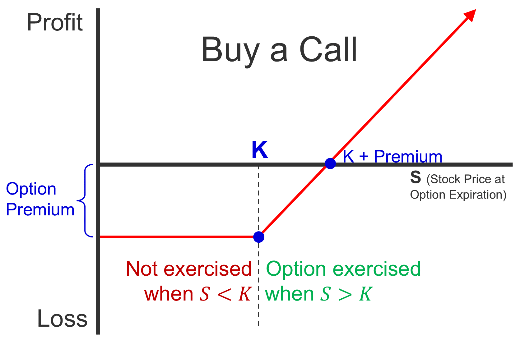
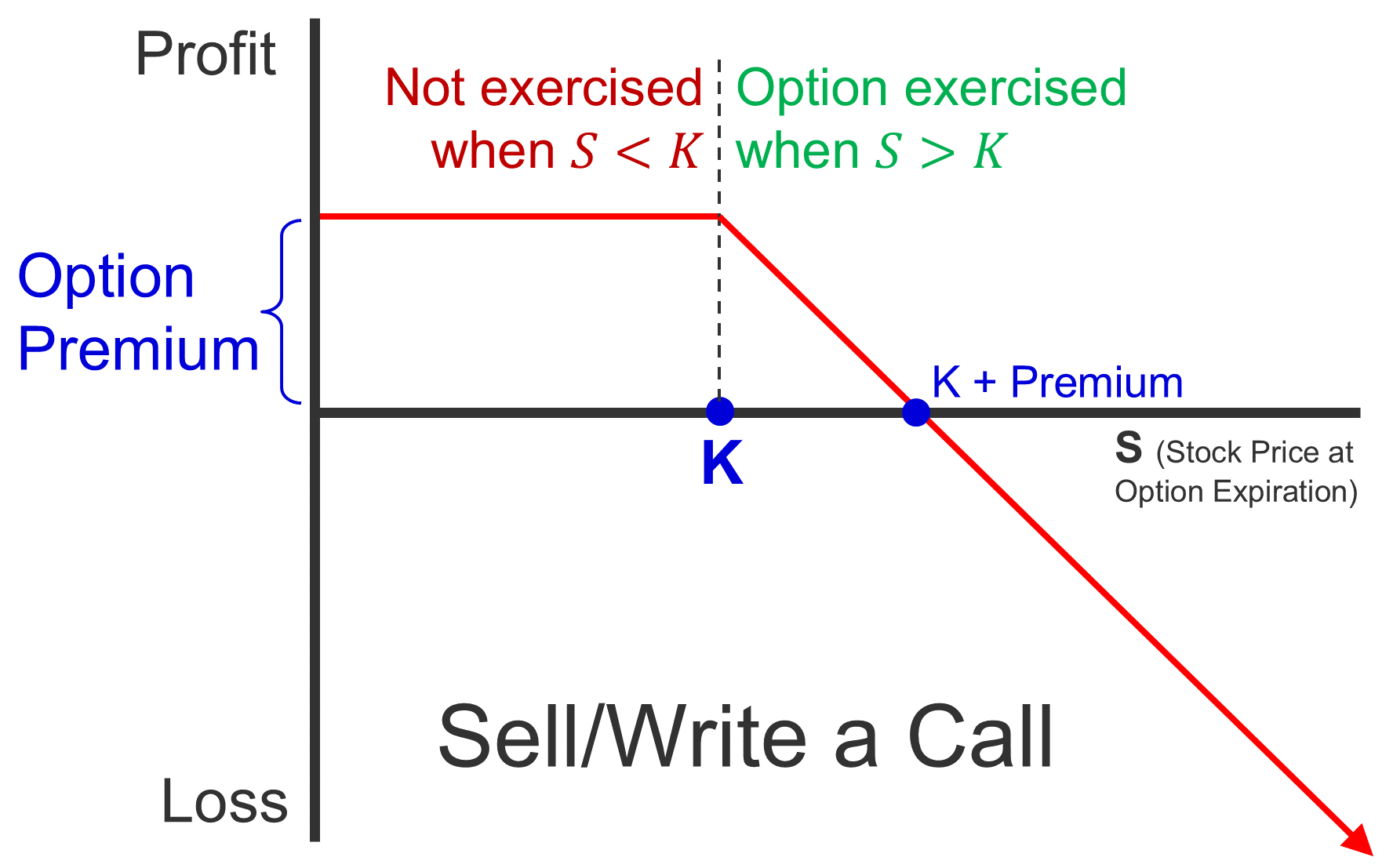
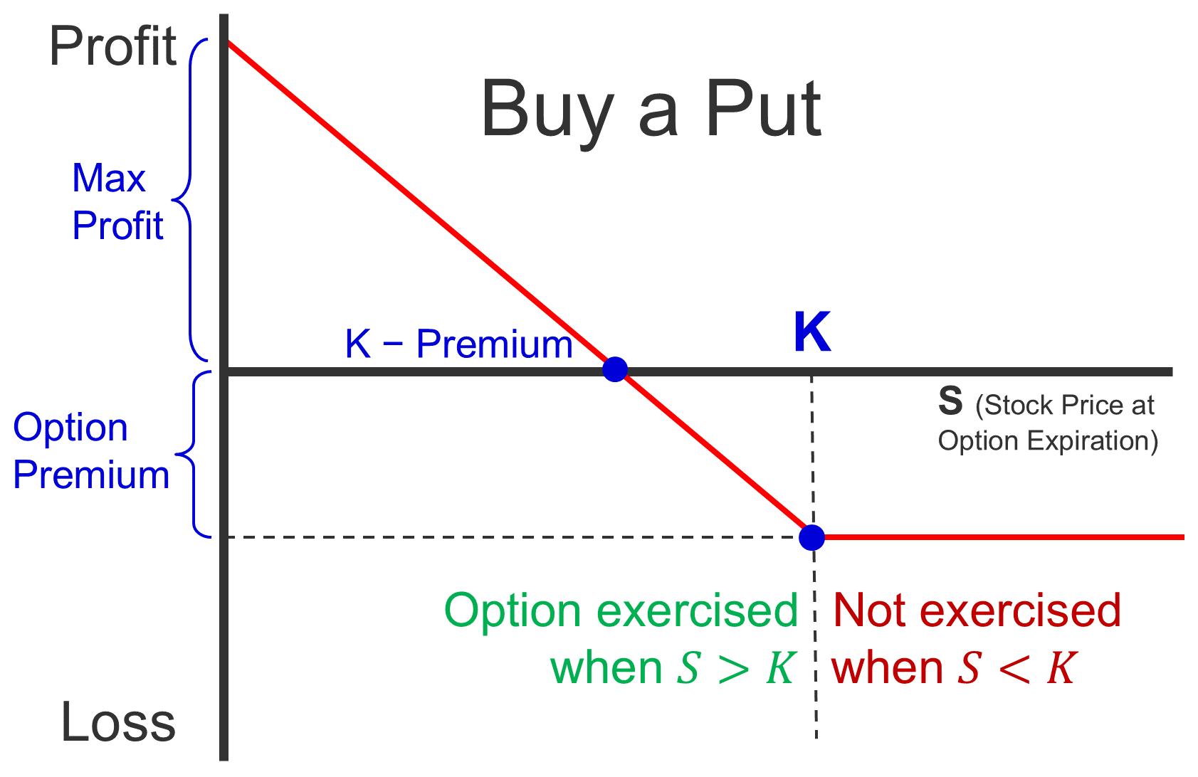
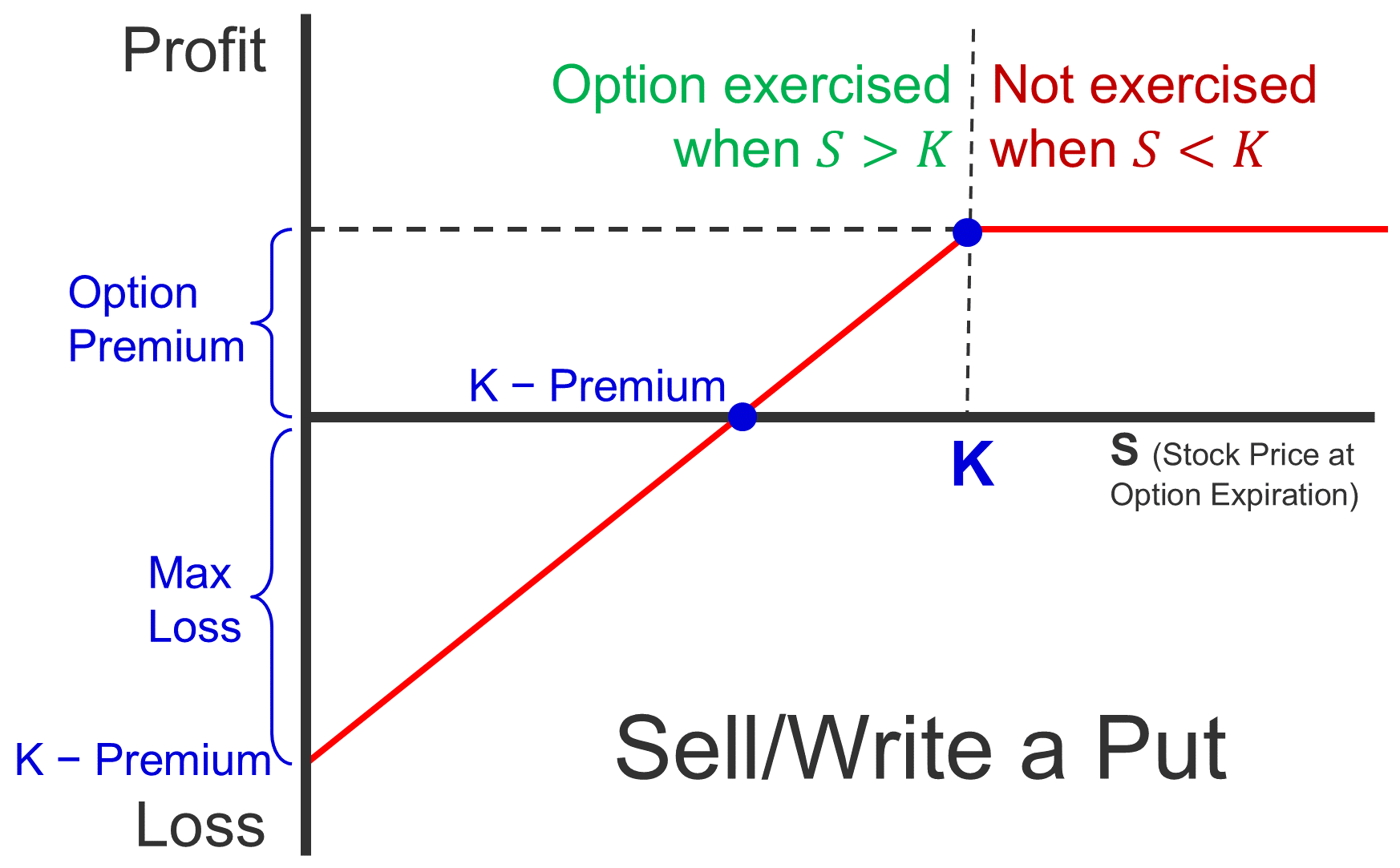
① IV Formulas: Call IV = Max ( S − K , 0 ) = \text{Max} (S-K, 0) = Max ( S − K , 0 ) Put IV = Max ( K − S , 0 ) = \text{Max} (K-S, 0) = Max ( K − S , 0 )
② P/L Formulas: Buying = I V − P r = IV - Pr = I V − P r Selling = P r − I V = Pr - IV = P r − I V
Combining ① and ②:
Buying a Call = Max ( S − K , 0 ) − P r = \text{Max} (S-K,0) - Pr = Max ( S − K , 0 ) − P r Buying a Put = Max ( K − S , 0 ) − P r = \text{Max} (K-S, 0) - Pr = Max ( K − S , 0 ) − P r Selling a Call = P r − Max ( S − K , 0 ) = Pr - \text{Max} (S-K, 0) = P r − Max ( S − K , 0 ) Selling a Put = P r − Max ( K − S , 0 ) = Pr - \text{Max} (K-S, 0) = P r − Max ( K − S , 0 )
Premium = Intrinsic Value + Time Value
Leverage = Share Price×100 / Premium×100
Buy/Long Write/Sell/Short Call Put
References: 11 Apr 21.ppt and L11 Notes
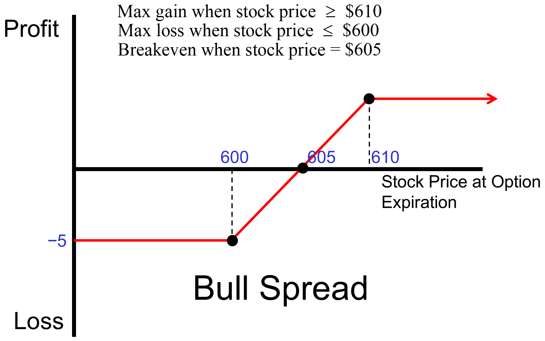
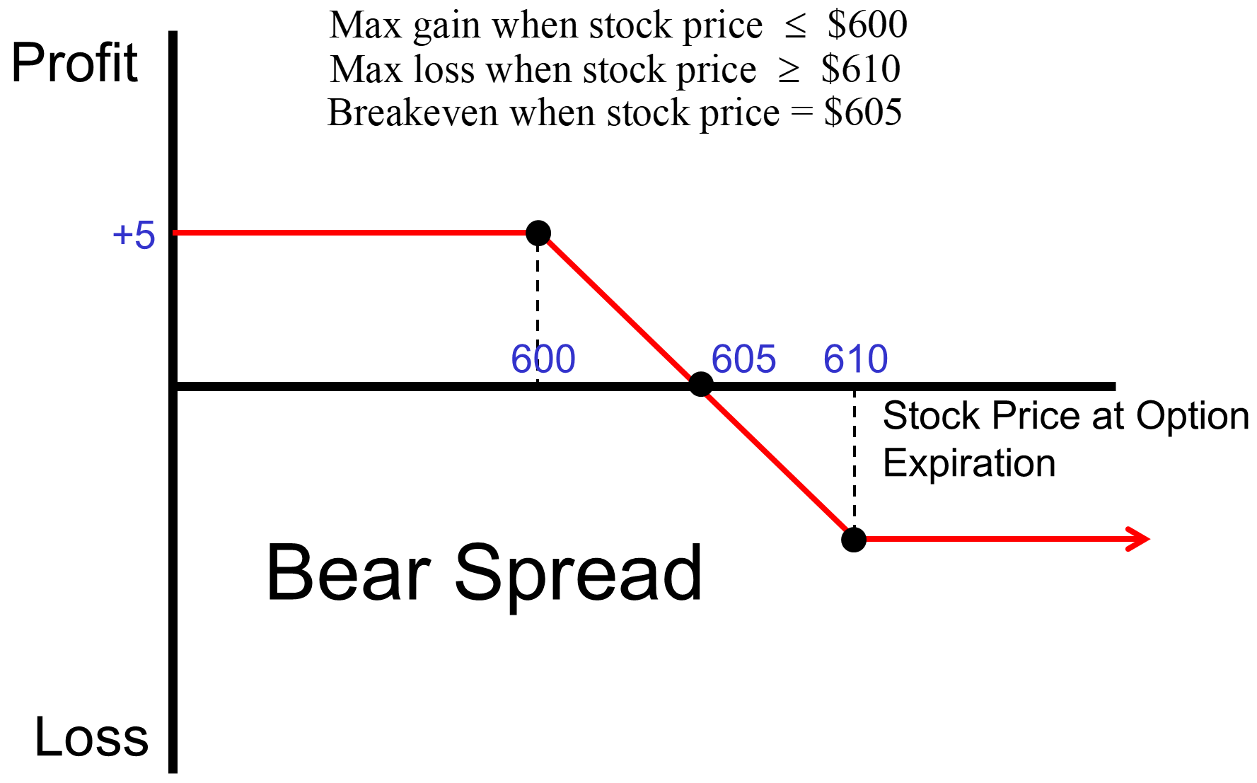
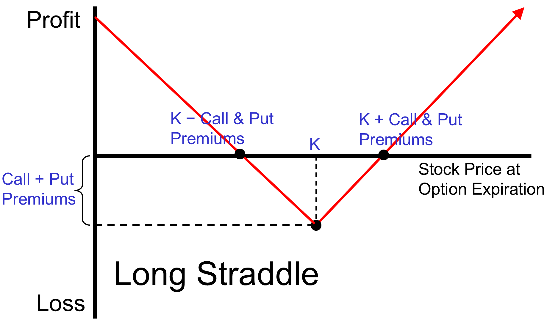
Spreads Straddles S will be relatively high . Construction: Buy a call with lower strike price and sell a call with higher strike price. S will be relatively low . Construction: Sell a call with a lower strike price and buy a call with a higher strike price. high volatility.Construction: Buy a call and a put with the same strike price. low volatility.Construction: Sell a call and a put with the same strike price.
References: 12 Apr 28.ppt , and L12 Notes
Δ Price = ( NewPrice − OldPrice ) \Delta\text{Price} = (\text{NewPrice} - \text{OldPrice}) Δ Price = ( NewPrice − OldPrice ) P / L = ∆Price × ContractSize P/L = ∆\text{Price} × \text{ContractSize} P / L = ∆ Price × ContractSize P / L = − ∆Price × ContractSize P/L = -∆\text{Price} × \text{ContractSize} P / L = − ∆ Price × ContractSize ContractSize = 5000 bushels wheat \text{ContractSize = 5000 bushels wheat} ContractSize = 5000 bushels wheat ContractSize = $50 per point of S&P 500 \text{ContractSize = \$50 per point of S\&P 500} ContractSize = $50 per point of S&P 500 Value of contract = ContractPrice × ContractSize \text{Value of contract} = \text{ContractPrice} × \text{ContractSize} Value of contract = ContractPrice × ContractSize Leverage = Value of Contract Initial Margin \text{Leverage} = \frac{\text{Value of Contract}}{\text{Initial Margin}} Leverage = Initial Margin Value of Contract
References: 13 Dec 2.ppt , L13 Notes
© 2026 Rob Munger